Conditional row color based on a cell value

Jeremy (US) asked me a question about coloring based on a cells value:

First your product ASAP Utilities is great and has been a life saver. One feature that would be outstanding is a conditional row color based on a cell value.
For instance there are numerous times I have to color a row because the value of a cell in a column is set either TRUE of FALSE or 0 or 1 and I currently do this by hand review.
If the ASAP utilities has a way to do this already I would love to know how.

Excel has a great built-in function to achieve this: Conditional Formatting (In the menu Format » Conditional formatting). The first time it might be a little difficult to find your way to do this but if you spend a little time with it you will soon realize it is powerful function.

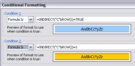
In the following example if we want the rows to be colored blue when column C is true and orange if the value is 1, we can use the following formula's:
Select all the cells that need to be colored. Usually we color a cell based an its value and use the [Cell Value Is ] in the conditional formatting box. To format cells based on other cells you need the [Cell Formula Is].
We use the =INDIRECT() function to get the value of column C for each row:
If the value is TRUE : =INDIRECT("C"&ROW())=TRUE
If the value is 1 : =INDIRECT("C"&ROW())=1
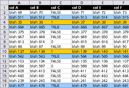
The result:

Download the example workbook

Interesting links:
http://www.cpearson.com/excel/cformatting.htm
http://www.contextures.com/xlCondFormat01.html

A "quick and dirty" method is using:
ASAP Utilities » Select » Conditional row and column select, hide or delete
and then color the selected rows.

109 comments

Neil

great info, but I have something a little more complicated here…

In Column A I have "Date Checked In" and in Column B I have "Time Checked In". In column C I have the following formula used to have a "Call Back By" within 2 hours:

=DATE(YEAR(A3), MONTH(A3), DAY(A3))+TIME(HOUR(B3)+2, MINUTE(B3), SECOND(B3))

I've been trying this for awhile.. How can I conditionally format the row to highlight if the date/time in Column C exceeds the current time (i.e. NOW())?

Neil

Whoops, I meant "…if the current time exceeds the date/time in Column C"

Neil

I figured it out, just FYI. There has to be a reference cell; as an example, put A1 as:
=NOW()
column C just needs to be conditionally formatted to be:
>=$A$1

The trick is to have both cells formatted the same way, i.e. mm/dd/yyyy [h]:mm pm

Colleen

Thank you so much, I have been looking for this for weeks!

Mike

Please Help!

I have been using a row interval color change macro for a few years. I believe that it is the best tool that could help me with the following… I just can't find how.

I need a way for excel to do a color transition "count"….

I need excel to now count the number of interval row color changes (transitions)… not a row count, but a row group count based on color (4 rows, then three rows, then one, then, one, etc – no pattern – I use a two color transition).

I do this manually by numbering only the first row color change… there has to be a way to tell excel to do this, no?

background:
I use access and pull a table into excel which has a list of items applied for by address.

If someone applies for 3 things on an application (they applied or requested something), it gets entered as 3 items creating 3 records and 3 rows on a table.

Lets say that typically there is no pattern to the number of items being requested on a single application –

To actually "see" how many items were entered from a single application, sort by record # (order entered)- highlight interval rows by address – this is how I can tell groups of rows were from one application, on the same day, from a single person.

My goal is to count the number of "applications" despite the number of "items/records/rows".

The data I'm working with goes back to '89 and these items have never been "linked" together as originating from a single application. The only way I can see their grouping is through the highlight row intervals as the data changes.

OK – now I want to count the INTERVALS. I want a count of applications.

My spreadsheet has 2 colors – blue and yellow. I might have 4 yellow rows, then 2 blue, then single row transitions for a while… etc.

IS THERE A WAY FOR EXCEL TO COUNT THE "CHUNKS" OF COLORED ROWS (not a row count – but an interval or color transition count)???

Nick Wigston

Works perfect, best answer on the web

NICK

=INDIRECT("AM"&ROW())=R

tHE FORMULA YOU TYPED CONTAINS AN ERROR

Bastien

Hello Nick,

If it is your own formula to which you are referring, then you should put quotes around the letter R, then you can use it in the formula:
=INDIRECT(”AM”&ROW())="R"

Kind regards,
Bastien Mensink

Prabakar

Thanks a lot.

NEY

thank you a lot for this post.

Rizwan

Thanks……….
Was looking for this for long time……

Hein

Hello Bastien,

Thanks for this post, it has been incredible helpful to me. Took me a little while to realize that I had to insert quotes when setting an own value.

After almost 5 years still helpful!
Thanks, again!

Cheers,
Hein

Andric

Is there any possible way to make this happen if instead of the value being "true" or "0", it's anything i put on the cell??
Thank you

Bastien

Hello Andric,

Yes you can. The possibilities are almost endless.
For example if you want cell A1 to be colored when it is isn't empty, you can use the following formula as conditional formatting:
=ISBLANK(A1)=FALSE

The following article might be interesting to you:
http://excel.tips.net/Pages/T002800_Shading_a_Cell_Until_Something_is_Entered.html

Kind regards,
Bastien Mensink

ABN Barbosa

Olá Bastien Mensink!

Não estou conseguindo, deixar a linha completa de todos funcionarios DENITIDO(S) (A1) e (A3) com cor Vermelha, usando =indireto("A"&Row())=Demitido

A B C
Situação Adm/Demissão Funcionário

1 Demitido 01/08/2010 Roberto
2 Ativo 01/05/2007 Maria
3 Demitido 15/09/2010 José
4 Ativo 05/02/2005 João

OBS: Caso possa fazer um exemplo no excel 2007, e enviar para meu e-mail.

Desde já, antecipo meus agradecimento.

ABN Barbosa

Tom Murphy

Thanks for this blog post. Was really helpful with a spreadsheet I was working with. Keep up the good work!

dian

It is really great but can you tell me if I want to color the full row for a specific number or text…I think you are not getting what I want to say…it's like..
** If my sheet found any "0" or say text like " mona" in a row it will color the full row yellow…..
** If my sheet found any "1" or say text like " lona" in a row it will color the full row green…..

Is it possible with conditional formating????? I am searching it for a long time..

ahmed

can anyone tell me how to make row change color if i put date (12.12.2009) in cell???
i tried this:
=INDIRECT(”C”&ROW())=DATE
=INDIRECT(”C”&ROW())=dd/mm/yyyy and similar,
but nothing is working?
please i need it as soon as possible

Josh

@ahmed
If Col C only has dates in it and you want them to be colored when this is keyed in try
=INDIRECT(”C”&ROW())>1

this will colour it when you key in any numeric value greater than one and as excel stores dates as numbers it will colour this when a date on or after the 2/1/1900 is keyed in, this can be also be used to only highlight cells after a certain date.

=INDIRECT(”C”&ROW()>40477 will colour cells with a date from today onwards. to find out what numbers dates convert to key in the date and then change the cell format to number.

Leo

This page was SO helpful THANK YOU!!!

bOBBy

Can this function help with finding duplicate value in a column and color the rows with duplicate columns. So if c1=c2 then one color for the whole row, if c2 is not equal to c3 then second colr

Bastien

Hello Bobby,

Yes, it surely can.
The following article from MS shows how you can use conditional formatting to find duplicates.
It uses that =COUNTIF() formula to do that:
http://office.microsoft.com/en-us/excel-help/locate-duplicates-by-using-conditional-formatting-HA001136616.aspx

Note:
The =COUNTIF() function as a few limitations. It only compares the first 15 digits or numbers so it wouldn't work for creditcardnumbers because it believes that 4916685766246816 and 4916685766246813 are equal. And it returns an error if one of the cells has a length of more then 255 characters.
The article below is about Excel 2000, but these limits are still in Excel 2010:
http://support.microsoft.com/kb/231114
Usually you won't run into this limits, but it might be good to know that they are there.

If you have such numbers or large values then you can use the "duplicate" tools from ASAP Utilities because those do not have that limitation.

Kind regards,
Bastien Mensink

Angel

hi,
I want to color a cell based on the text in the adjacent left cell.
ie, if cell C1 has the text "Closed", i want the cell D1 to be in green color.
And this needs to be applied to all the cells in column C and D.
Is this possible?

Elliot

Hi,

I am trying to change the colour of 5 cells which are in a row, when the value of another cell is equal to a certain phrase.

For Example:

If Cell B1 contains the phrase Existing Accounts the colour of Cells S1:W1 change

Can you help?

Thanks
Elliot

Bastien

Hello Angel and Elliot,

Both of these can be done.
If you want a cell to change color, you have to set up the conditional formatting in that cell.
I don't have the time to work out specific examples for your but if you experiment with it and take a look at the mentioned websites I'm sure you'll get it working.

Kind regards,
Bastien Mensink

Sylvia

I don't know why it took so long and I had to wade through all kinds of unhelpful websites till I finally found your "one in a million"! It worked immediately and I am so thankful! I never saw anyone else refer to this INDIRECT function. THANK YOU THANK YOU THANK YOU!!!!!

Miriam W

@ Helen: The formula would need to include AND(Indirect(…)30), with the “…” being your reference cell formula.

@ Marc: You would need to have something like the Index function if the cells are not the same, but if you are trying to make it for the cell itself, you can use isblank(indirect(“E”&row()))

@ Neil: You just need a simple, if the cell with the date is greater than now() in the conditional field. Something like indirect(“C”&row())>now()

@Nick: When you say =R, R needs to be in double quotes

@Angel: Just put in indirect(“C”&row())=”Closed” as your argument. Make sure you have set your formatting to what you need it to be.

@Elliot: That is super, super easy. Say the cell is B5, your argument would be $B$5=”Existing Accounts”

@ everyone/all readers
Bastien is NOT here to solve all of your problems for you. He has created a helpful site that shows a technique not many even know about. Be grateful and do a bit of trial and error on your own spreadsheets. I have seen many of these equations that everyone is asking for easy to figure out with a bit of trying. Just remember that your argument must return true or false. If you cannot put IF() around it, it isn’t going to work.

@ Bastien: Thank you. I was looking for a way to do Index() in it and I was not quite understanding how conditional formatting worked. I really appreciate the instruction.

Charity

I am wanting to auto Change the text color from red to black in Col A rows 2 through 33 based on the value of Columns B, C, E and G rows 2 – 33 being greater than 0.

How do I go about doing this? I don't want this format in any other cells/rows except the ones stated above.

I'm not excel savy so please explain in detail lol.

Thanks in advance!

Excel 2007 Conditional Row Formatting « just samson

[…] some knowledge of writing formulas and knowledge of the INDIRECT function. Bastien blogged about Conditional row color based on a cell value which illustrates the process quite nicely. The steps I am about to cover mimic Bastien's […]

Troy

jeez. thank you. took me forever to find this answer on google. should be top results.

Jen

BRILLIANT! Thank you so much for posting this. I've searched all over for the answer to this question, and your solution is the only one I've seen that works. It works!

Waz

All great stuff…

Any help with this one would be greatly appreciated…

I have been using the =INDIRECT("A"&ROW())="variable" rule in the past to colour an entire row, with 'variable' being whatever cell content I want to command the rule.

I now want to apply the same rule, but only if either an odd or even number is in the cell, rather than stating a fixed variable.

Any thoughts???

Thanks

jomobe

AWESOME! Months of searching for a way on my own to do this and viola'. My answer is right here. I had to play but here's what I did (Oh, I'm no expert by far):
Excel 2003, conditional formatting, spreadsheet of text, numbers and dates with headered columns and named rows

I wanted to shade an entire row of data (the data only) if the text in a specific cell (column based) in that row contained specific text.

The formula that worked for the conditional formatting is =INDIRECT("column letter"&ROW())="text"

I highlighted my entire data table with header row;
ALT+O (format), D (conditional);
Condition 1: FORMULA IS;
=INDIRECT("C"&ROW())="Not";
Click the FORMAT button and set PATTERN desired;
Click OK;
Click OK.

Explanation:
=indirect – Use INDIRECT when you want to change the reference to a cell within a formula without changing the formula itself.

("C"&ROW()) – the "C" is the column label, not the header title. The &ROW will apply the format to the entire row and the () limits the format to within your highlighted area
="text" – the text is the content of the cell in column C. In my case, it looked like ="Not" where Not is the text I enter into the cell to close out the row.

Now when I open my spreadsheet, all of the closed out rows with Not in column C are highlighted, or colored to give the quick representation. I still filter my data table, but this allows the overall appraisal of progress.

I hope this helps someone else like me.

Thanks to all of the contributors to this post,
jomobe

jomobe

Hey WAZ,

Try using =MOD($A1,2)=1

You will be abe to set your formatted area by highlighting your cell array first;
MOD is an odd one but works for what you stated;
$A1 will look at the cell with your numbers based on the entire column and the ,2 I'm not sure because 0 and 1 do not work at all;
the =1 will format the entire row of data that an odd number shows up in and =0 will for mat the row for even numbers found. Again, 2,3,4,… does not work at all.

Hope this helps …
jomobe

leonard

tnx.. . it really helps! now i can make my worksheet more comprehensible, time saving and more conveying!

Staci

I have a spreadsheet and when i enter something into one column i want to change the color of the entire row.
they are currently yellow until that column has something entered into it which i put in manually and would like it to do it automatically.
please if anyone knows how to do it and give me exact instructions to follow that would be so helpful.
thanks!

Hari

Hi,

I need to highlight a row if the difference between two column ( column will have dates ) is greater than 1. Also I need to replace today's date if the second ( date ) column is empty and it should be hidden.. Please suggest.

Best regards,

Hari Bhaskar.

DANA

hello!

jomobe, your post was really useful and im mch closer to getting what i want…but not quite…maybe someone can help!

i used the exact formula, but replaced the "not" with "n"

=INDIRECT("C"&ROW())="N";

what i want though, is for the entire row to be highlighted if the cell in coloums C *AND* the cell in coloumn D ="N" …
Basically, its not enough for the row to be highlighted if its just one N…

im not that experienced with excel and have tried everything i know, so any help would be HUGELY appreciated!

thanks!

Dana
i hope that makes sen

Stuart

Hello

I used the formula

=INDIRECT("J"&ROW())="YES" and made it go yellow

however i want to do another saying

=INDIRECT("L"&ROW())="YES" and made it go red

with the second overwriting the first how do i make this work?

thanks

Stuart

VARUN

in Excel 2007 I need to conditally format a row (fill with color) based on text rather than a numeric value. I have one worksheet and I need the rows highlighted with differernt color based on Approved,not approved, I can't seem to get the formula right to get the entire row highlighted. When I say "Approved " it only highlights that cell and not the entire row… Any suggestions pl let me know.

Bastien

Hello Varun,

Thank you for your feedback.
If you want the entire row to be colored, then you have to set the conditional formatting for each cell in that row.
Just select the entire row and then set the conditional formatting conditions.

Kind regards,
Bastien

Sufyan

Hi

I have a problem which i still havent been able to overcome. I am using excel 2007.

i need the entire row to be highlighted by a specific colour based on the value of one cell in that row. Ex. if the cell contains the text "completed", i would want the entire row to get colored.

I could do this using conditional formatting using value of the cell option for the entire row to get highlighted.

PROB: i want this conditional formatting to be repeated in all the rows below that too… Have a couple of hundred rows, and this keeps getting added. Is there any way to copy the conditional formatting to below rows too??

Very much in need of help.

Thanks,

Sufyan

Bastien

Hello Sufyan,

Thank you for your feedback.

Yes, you can copy the conditional formatting, just like normal formatting.
Just copy the row, select the target row and choose in the Excel menu Edit > Paste special > Formats
or in the Excel ribbon Home tab > Paste > Paste special > Formats

Kind regards,
Bastien Mensink

Mayur

Hi Bastien,
I am using 2003, Ihave created a drop down list with four options & i want all the 4 in diff colours. Whenever any option is selected it has to appear with the respective assigned colour. Kindly assist.

Bastien

Hello Mayur,

Thank you for your comment.
I'm sorry but that is not possible, neither in Excel or via ASAP Utilities.

Kind regards,
Bastien Mensink

Yaron Berlinsky

Thanks.
Great tip.
Solved issue for me.

Matt

For the poster wanting to know how to format an entire column based on one row's value in that column, I got it to work. If you want to format the column something whenever the column value in row 1 = "H", use this for the conditional formula:
=A$1="H"

if you're looking in row 2, use:
=A$2="H"

etc

Sharan

Im trying to apply conditional formatting in Excel 2010 for a defect report. I’m tryi8ng to change color of row based on the values present under the status column. For instance if the status value (in my case Column I) = “In progress” then im trying to make the entire row that has the value green.

I tried this selected the entire report and used this formula under Conditional Formatting ->New Rule->Use formula to determine which cell to format->Formula values where this value is true and entered the below value

=INDIRECT("I"&ROW())=Closed

This did not work for me , Can you please help me with this issue?

Bastien

Hello Sharan,

Thank you for your feedback.
You should put the text in quotes: =INDIRECT("I"&ROW())="Closed"
You can download an example workbook from:
//www.asap-utilities.com/blog/wp-content/Highlight-closed.xlsx

Kind regards,
Bastien Mensink

Sharan

It worked. Thanks a lot for following up!

Regards,
Sharanya.